Please Note: This article is written for users of the following Microsoft Excel versions: 97, 2000, 2002, and 2003. If you are using a later version (Excel 2007 or later), this tip may not work for you. For a version of this tip written specifically for later versions of Excel, click here: Creating 3-D Formatting for a Cell.
Written by Allen Wyatt (last updated September 8, 2022)
This tip applies to Excel 97, 2000, 2002, and 2003
Do you want the formatting of a cell to "stand out" from the surrounding cells? It's rather easy to do, once you understand how to create the illusion of three dimensions. Follow these steps:
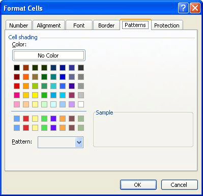
Figure 1. The Patterns tab of the Format Cells dialog box.
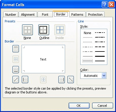
Figure 2. The Border tab of the Format Cells dialog box.
The cell you selected in step 1 should now look as if it is "raised" off the worksheet around it. You can accentuate the effect even more if you apply a background color to the cells that surround the one that you want to look raised.
ExcelTips is your source for cost-effective Microsoft Excel training. This tip (3061) applies to Microsoft Excel 97, 2000, 2002, and 2003. You can find a version of this tip for the ribbon interface of Excel (Excel 2007 and later) here: Creating 3-D Formatting for a Cell.
Program Successfully in Excel! John Walkenbach's name is synonymous with excellence in deciphering complex technical topics. With this comprehensive guide, "Mr. Spreadsheet" shows how to maximize your Excel experience using professional spreadsheet application development tips from his own personal bookshelf. Check out Excel 2013 Power Programming with VBA today!
A handy way to store latitude and longitude values in Excel is to treat them as regular time values. When it comes around ...
Discover MoreKeyboard shortcuts can save time and make developing a workbook much easier. Here's how to apply the most common of ...
Discover MoreNeed to cram a bunch of text all on a single line in a cell? You can do it with one of the lesser-known settings in Excel.
Discover MoreFREE SERVICE: Get tips like this every week in ExcelTips, a free productivity newsletter. Enter your address and click "Subscribe."
There are currently no comments for this tip. (Be the first to leave your comment—just use the simple form above!)
Got a version of Excel that uses the menu interface (Excel 97, Excel 2000, Excel 2002, or Excel 2003)? This site is for you! If you use a later version of Excel, visit our ExcelTips site focusing on the ribbon interface.
FREE SERVICE: Get tips like this every week in ExcelTips, a free productivity newsletter. Enter your address and click "Subscribe."
Copyright © 2024 Sharon Parq Associates, Inc.
 Please Note:
This article is written for users of the following Microsoft Excel versions: 97, 2000, 2002, and 2003. If you are using a later version (Excel 2007 or later), this tip may not work for you. For a version of this tip written specifically for later versions of Excel, click here:
Please Note:
This article is written for users of the following Microsoft Excel versions: 97, 2000, 2002, and 2003. If you are using a later version (Excel 2007 or later), this tip may not work for you. For a version of this tip written specifically for later versions of Excel, click here:
Comments